Descriptive Statistics
- Population: The entire group you want to study.
Example: All the students in a university. - Sample: A smaller group selected from the population.
Example: 100 students randomly chosen from the university. - Parameter: A numerical value that describes a characteristic of a population.
Example: The average height of all students in the university (e.g., 5.7 feet). - Statistic: A numerical value that describes a characteristic of a sample.
Example: The average height of the 100 students in the sample (e.g., 5.5 feet). - Mean (μ or x̄): The average of a set of numbers.
Example: For the numbers 2, 4, 6, the mean is (2 + 4 + 6) / 3 = 4. - Trimmed Mean: The mean calculated after removing a specified percentage of the smallest and largest values.
Example: For the dataset 1, 2, 3, 4, 100, if you trim 20%, you would remove 1 and 100, and then the trimmed mean would be (2 + 3 + 4) / 3 = 3. - Median: The middle number in a sorted list of numbers.
Example: In the list 1, 3, 3, 6, 7, 8, 9, the median is 6.- Even Occurrence
- Odd Occurrence
- Mode: The number that appears most frequently in a set.
Example: In the list 1, 2, 2, 3, 4, the mode is 2. - Variance: The average of the squared differences from the mean, another way to measure spread.
Example: If the heights are 5, 6, and 7 feet, the variance helps us understand how much these heights differ from the average height.- Variance measures how far each number in a set of data is from the average (mean).
- To do this, we first find the difference between each number and the average. If we just added these differences together, some would be positive and some would be negative, which could cancel each other out and make it seem like there’s no spread at all.
- By squaring these differences, we turn everything into positive numbers. This way, we can see how much each number varies from the average without any cancellation happening.
- Squaring also makes bigger differences count more, so it gives us a better idea of how spread out the numbers are.
- So, squaring helps us measure the spread while keeping everything positive and meaningful!
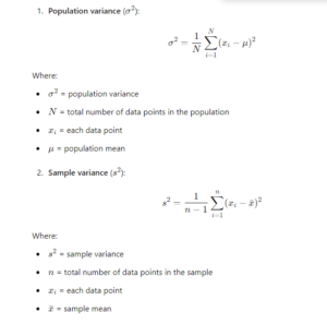
- Key Differences:
- Population variance divides by NNN (the total population size).
- Sample variance divides by n−1n-1n−1 (degrees of freedom) to account for bias when estimating the population variance from a sample.
- Standard Deviation (σ or s): A measure of how spread out the numbers are from the mean.
Example: If the heights of students are close to the average, the standard deviation is small; if they are very different, it’s large.- Key Differences:
- Variance is a measure of spread in squared units of the original data.
- Standard deviation is the square root of variance, so it brings the measure back to the original units of the data.
- Key Differences:
- Standard Error: What is Standard Error (SE)?
- Standard Error is the measure of how much the sample mean is expected to vary from the population mean (μ) due to the fact that we’re using a sample, not the whole population.
- Why do we calculate SE?
- When you’re working with samples, the sample mean can vary from sample to sample. The SE helps to account for this variability.
- SE gets smaller as the sample size (n) gets larger because larger samples provide more precise estimates of the population mean.
- In hypothesis testing or confidence intervals:
- When using a sample (not the entire population), you calculate the Z-score using the Standard Error instead of just the standard deviation.
- SE is smaller than σ, and as you mentioned, this makes the Z-scores larger (since the denominator is smaller) and helps better estimate the probability that the sample mean represents the population mean.
- Standard Deviation (σ) measures the variability of individual data points in the population.
- Standard Error (SE) measures the variability of sample means around the population mean.
- SE is smaller than σ, meaning sample means are less spread out than individual data points.
- When using a sample, SE helps to adjust the Z-score or other calculations to account for the smaller variability in sample means.
- Coefficient of Variation (CV): The ratio of the standard deviation to the mean, expressed as a percentage.
Example: If the average test score is 80 and the standard deviation is 10, the CV is (10/80) × 100 = 12.5%. - Percentiles and Quartiles: Percentiles divide data into 100 equal parts; quartiles divide it into four.
- Percentile: If you score in the 90th percentile on a test, you did better than 90% of test-takers.
- Quartiles: The first quartile (Q1) is the value below which 25% of the data falls.
- Skewness: A measure of the asymmetry of a distribution.
- Positive Skew: Most data points are low, with a few high outliers (e.g., incomes).
- Negative Skew: Most data points are high, with a few low outliers.
- Symmetric: The data is evenly distributed around the mean.
- Kurtosis: A measure of the “tailedness” of a distribution.
- Leptokurtic: More outliers than a normal distribution.
- Mesokurtic: Similar to a normal distribution.
- Platykurtic: Fewer outliers than a normal distribution.
- Outliers: Data points that are significantly different from the rest.
Example: In test scores of 70, 75, 80, and 30, the score of 30 is an outlier.- Detection Methods:
- IQR Rule: An outlier is any value below Q1 – 1.5 × IQR or above Q3 + 1.5 × IQR.
- Z-Scores: A score that is more than 3 standard deviations away from the mean is typically considered an outlier.
- Detection Methods:
- Histogram: A graphical representation of the distribution of numerical data, using bars to show frequency.
Example: A histogram of test scores might show how many students scored in each score range. - Box Plot (Box-and-Whisker Plot): A graphical display of data that shows the median, quartiles, and outliers.
Example: A box plot can quickly show the spread and center of student scores, highlighting any outliers. - Frequency Measures
- Frequency Distribution: A summary of how often each value occurs in a dataset.
Example: In a survey of pet ownership, you might find that 20 people have dogs, 15 have cats, and 5 have birds. - Cumulative Frequency: A running total of frequencies, showing how many observations fall below a certain value.
Example: If 10 students score below 60, and 15 score below 70, the cumulative frequency for below 70 is 25 (10 + 15). - Relative Frequency: The proportion of the total number of observations that falls within a particular category, expressed as a percentage or fraction.
Example: If 30 out of 100 students score above 75, the relative frequency is 30/100 = 0.30 or 30%.
- Frequency Distribution: A summary of how often each value occurs in a dataset.
- Distribution
- Normal Distribution
- Standard Distribution
Inferential Statistics
Hypothesis Testing
- Null Hypothesis (H₀): The statement that there is no effect or no difference, which we aim to test.
Example: “There is no difference in test scores between two teaching methods.” - Alternative Hypothesis (H₁): The statement that there is an effect or a difference.
Example: “There is a difference in test scores between two teaching methods.” - p-value: The probability of obtaining results at least as extreme as the observed results, assuming the null hypothesis is true.
Example: A p-value of 0.03 means there is a 3% chance of observing the data if the null hypothesis is true. - Confidence Interval: A range of values used to estimate a population parameter, indicating the degree of uncertainty.
Example: A 95% confidence interval for the average height might be (5.5 feet, 5.9 feet), meaning we are 95% confident the true average height falls within this range. - Confidence Level: The percentage of times the confidence interval would contain the true population parameter if you repeated the experiment many times.
Example: A 95% confidence level means if we took many samples, 95% of the calculated intervals would contain the true population mean. - Error in Hypothesis
- Type I Error (False Positive): Rejecting the null hypothesis when it is actually true.
Example: Concluding that a new drug is effective when it actually is not. - Type II Error (False Negative): Failing to reject the null hypothesis when it is actually false.
Example: Concluding that a new drug is not effective when it actually is.
- Type I Error (False Positive): Rejecting the null hypothesis when it is actually true.
- Power of a Test: The probability of correctly rejecting a false null hypothesis.
Example: A power of 0.8 means there is an 80% chance of detecting an effect if there is one. - Effect Size: A measure of the strength of a relationship or the magnitude of an effect.
- Cohen’s d: Measures the difference between two group means in terms of standard deviation.
- Pearson’s r: Measures the strength and direction of the linear relationship between two variables.
- Degrees of Freedom (df): The number of independent values or quantities that can vary in an analysis without violating any given constraints.
Example: In a t-test with 10 samples, df = 10 – 1 = 9.
Statistical Tests
- t-test: A test used to compare the means of two groups.
Example: Comparing the test scores of students taught by two different methods. - z-test: A test used to determine if there is a significant difference between sample and population means when the sample size is large.
Example: Testing if a sample mean height of 5.6 feet significantly differs from a population mean of 5.7 feet. - ANOVA (Analysis of Variance): A statistical method used to compare means among three or more groups.
Example: Testing if students from three different schools have different average test scores. - Chi-Square Test: A test used to determine if there is a significant association between categorical variables.
Example: Testing if there is a relationship between gender and preference for a type of music. - F-Test: A test used to compare the variances of two populations.
Example: Testing if two different teaching methods have different levels of variability in test scores. - Levene’s Test: A test to assess the equality of variances for a variable calculated for two or more groups.
Example: Checking if the variances of test scores among different classes are equal. - Shapiro-Wilk Test: A test used to check if data follows a normal distribution.
Example: Testing if a set of student scores is normally distributed before applying parametric tests. - Post Hoc Test: Tests conducted after ANOVA to find out which specific group means are different.
Example: If ANOVA shows significant differences among three groups, a post hoc test will identify which groups differ.
Regression and Correlation
- Regression: A statistical method used to understand the relationship between dependent and independent variables.
Example: Predicting a student’s final grade based on their study hours using a regression line. - Correlation: A measure of the strength and direction of the relationship between two variables.
- Positive Correlation: As one variable increases, the other also increases (e.g., more study hours lead to higher grades).
- Negative Correlation: As one
